Deformable Conv v1
这篇文章其实比较老了,是 2017 年 5 月出的
Motivation
Task 上的难点
视觉任务中一个难点就是如何 model 物体的几何变换,比如由于物体大小,pose, viewpoint 引起的。一般有两类做法:
- 在数据集上做文章,让 training dataset 就包含所有可能的集合变换。通过 affine transformation 去做 augmentation
- 另一种就是设计 transformation-invariant (对那些几何变换不变)的 feature 和算法。比如 SIFT 和 sliding window 的方式。
文章说上述两种方式有问题,几何变换我们是事先知道的,这种不能 generalize 到其它场景和任务中。以及 hand-crafted 的设计适应不了负责场景。
CNN 的缺陷
对于geometric transformation 的问题,目前的 CNN 主要是通过 data augmentation 和一些手工设计,比如 max-pooling 解决的(max-pooling 只能解决一些很小程度的变化,比如字母 A 稍微倾斜了一下)。
CNN 的主要问题就在于它的采样操作是 fixed 的。每个点的 receptive field 是一样大的,对 high-level 的语义不太好。
Controbution & Details
主要提出了两个模块,Deformable Conv 和 Deformable Pooling。他们的优点是很方便的嵌入的已有的模型中,不需要额外的监督信号。
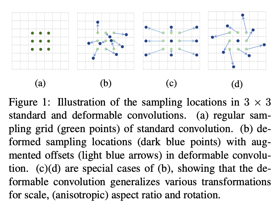
这张图很好的诠释了 deformable conv 是怎么做的
Deformable Convolution

这个操作很好理解,用另一个一样大小的卷积去学 offset, channel 数是 \(2N\)。 \(N\) 是 kernel 的面积。比如说,对于 3x3 卷积,也就是说每个 output 点,在 Input feature map 上都有 9 个点要算,\(N=9\), 对于每个点,都有 \(x\) 和 \(y\) 方向上的 offset。
这里的 \(N\) 实际上是 kernel 里的 sampling location 数。如果 3 x 3 的 kernel 的话,\(N = 9\)。 在deformable conv v2 的 paper 解释的比较清楚。
如果你去看它的代码的话,会发现它还有一个参数,叫 deformable_group, 这个参数在 paper 里是没有被提到了,具体的解释可以参考这个issue 回答。
The standard deformable group (dg=1) is position-depedent. It applies the same offset to all channels of one pixel. Similar to Group Normalization, it will have more flexibility with a larger dg since different channels are responsible for detecting different parts, and may have different geometric variations.
这里稍微不好想是怎么求反传导数
这里是 forward 的形式,之前的铺垫公式笔记简单,读者可自己看一下。这里,\(\Delta p\) 就是 offset。用 bilinear sampling 来计算任意位置的 feature 大小。反传公式在这里
注意:这里有一个非常非常非常容易混淆的点,所谓的deformable,到底deformable在哪?很多人可能以为deformable conv学习的是可变形的kernel,其实不是不是不是!本文并不是对kernel学习offset而是对feature的每个位置学习一个offset。
Deformable Pooling
ROI Pooling模块是two-stage中常见的池化方法,基于目标检测方法中所有的region proposal。将任意输入大小的矩形调整为固定尺寸大小的feature。给定input feature map x 和一个大小为\(w\times h\),位于左上角的区域\(P_0\),ROI Pooling将会把这个ROI划分为\(k\times k\)个bins,同时输出一个size为\(k\times k\) 的feature map y,可以用如下公式表示:
其中,\(n_{ij}\)是bin中像素的数量
有了这个基础,我们再来看可变形池化,公式如下:
相比普通ROI Pooling,同样增加了一个offset,下图为网络结构:具体操作为,首先,通过普通的ROI Pooling得到一个feature map,如下图中的绿色块,通过得到的这个feature map,加上一个全连接层,生成每一个位置的offset,然后按照上面的公式得到\(\Delta \mathbf{p}_{ij}\),为了让offset的数据和ROI 的尺寸匹配,需要对offset进行微调,此处不是重点。全连接层的参数可以通过反向传播进行学习。
由于按照RoI长宽比例进行水平和竖直方向偏移,因此每一个bin的偏移量只需要一个参数来表示,具体可以用全连接来实现。

之后还介绍了 position-sensitive(PS) ROI Pooling,也是有疑问,感觉作者想的非常不清楚。在 PS ROI pooing 里,先得到原图大小的 offset field, 那 ROI 里的一个小区域里的 offset 是怎么得到的?
def get_deformable_roipooling(self, name, data, rois, output_dim, spatial_scale, param_name, group_size=1, pooled_size=7,
                              sample_per_part=4, part_size=7):
    offset = mx.contrib.sym.DeformablePSROIPooling(name='offset_' + name + '_t', data=data, rois=rois, group_size=group_size, pooled_size=pooled_size,
                                                   sample_per_part=sample_per_part, no_trans=True, part_size=part_size, output_dim=output_dim,
                                                   spatial_scale=spatial_scale)
    offset = mx.sym.FullyConnected(name='offset_' + name, data=offset, num_hidden=part_size * part_size * 2, lr_mult=0.01,
                                   weight=self.shared_param_dict['offset_' + param_name + '_weight'], bias=self.shared_param_dict['offset_' + param_name + '_bias'])
    offset_reshape = mx.sym.Reshape(data=offset, shape=(-1, 2, part_size, part_size), name='offset_reshape_' + name)
    output = mx.contrib.sym.DeformablePSROIPooling(name='deformable_roi_pool_' + name, data=data, rois=rois, trans=offset_reshape, group_size=group_size,
                                                   pooled_size=pooled_size, sample_per_part=sample_per_part, no_trans=False, part_size=part_size, output_dim=output_dim,
                                                   spatial_scale=spatial_scale, trans_std=0.1)
    return output
Deformable Conv v2
说完了 v1, 聊一个新出的 v2。 Deformable Conv v1 貌似没有怎么调参,所以 performance 其实是不高的,在 v2 中他们的 performance 非常好了。发现 Naiyan Wang 在这篇对 v1 的文章里提到过这个建议,然后 v2 就采用了。
Motivation
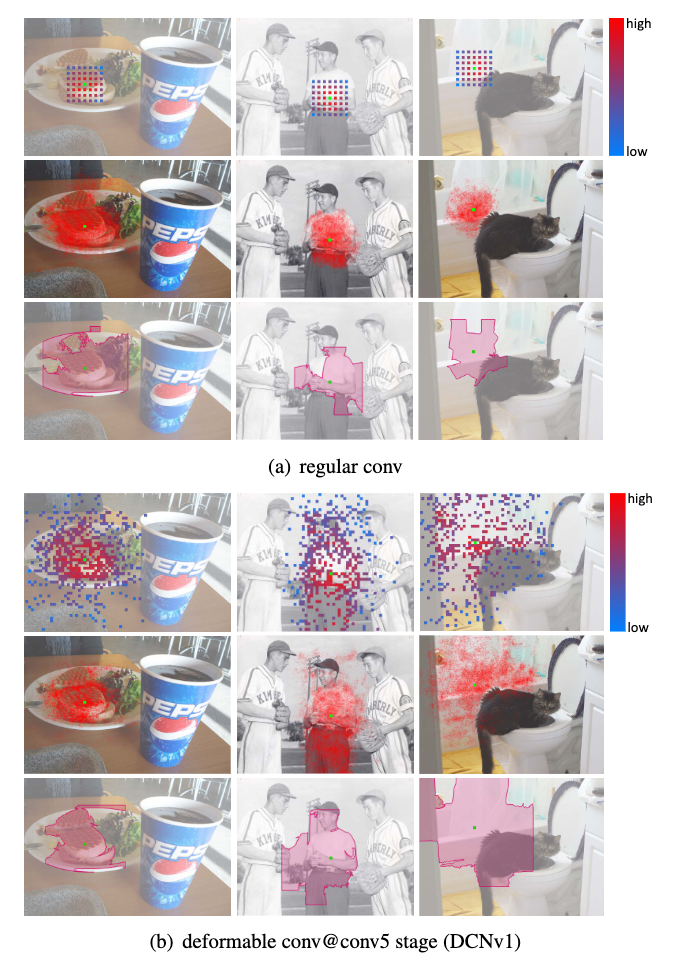
文章分析了 v1 版本中的问题,在使用了 deformable conv 后,还是会覆盖到 irrelevant context, 影响 performance。 所以 v2 的 contribution 基本上围绕如何消除 irrelevant context 的影响上。
为了分析 network 的 receptive field, 作者用了三个指标:
- Effective receptive fields: 它是看在原始 image 上,对每个 pixel 的扰动会对 node response 产生多大影响。
- Effective sampling / bin locations: 看对 sampling location 的扰动,能对 response 有多大影响。
- Error-bounded saliency regions: 能让 node 保持同样 response 的最小区域。在附录里,作者给了详细的介绍。
在 figure(1) 中,就可以看出他们的不同。
Controbution & Details
- 更多的 deformable conv
在 conv 3-5 都用了 deformable conv
- modulated deformable conv
为了减少 irrelevant 区域的影响,我们就想办法消除这些区域。通过学习 weight, 我们可以让这些区域的 weight 变得比较小。
所以在学习 offset 的同时,我们又学习一个权重。这个权重是对每个 location 不同的。同样的操作也适用于 deformable RoIpooling。
- R-CNN Feature Mimicking
mimicking 的方式也是为了避免 irrelevant 信息的影响,为什么会有 irrelevant 信息,因为我们的 receptive fields 比较大,会受到 object 周围信息的影响。但是在 RCNN 中,它的输入是 cropped patch, 这个 patch 已经将不少背景信息 remove 了,如果我们让 faster-rcnn 学出来的 feature 和这个 patch 得到的 feature 靠近,就可以一定程度上消除他们带来的影响。

上图是 mimicking 的网络。用 mimicking 的工作,很巧妙的把 inference 时间提快了。
Experiments
在标准的 mask-rcnn 上修改,替换成 modulated deformable conv 和 deformable RoIPooling。
注意这里 input image 的 short side 变成了 1000,figure 4 说明了这个。对于更多的图像,因为 network 层数是固定的,所以 receptive field 没有那么多,效果变差。
文章在后面还在 imagenet 上 pretrain 了,提供了基础模型。
Performance
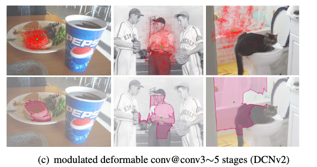
可以看到替换成 modulated deformable conv 后,区域更集中了。但是即使是 modulated conv, 还是会覆盖到一些 irrelevant 的物体上。