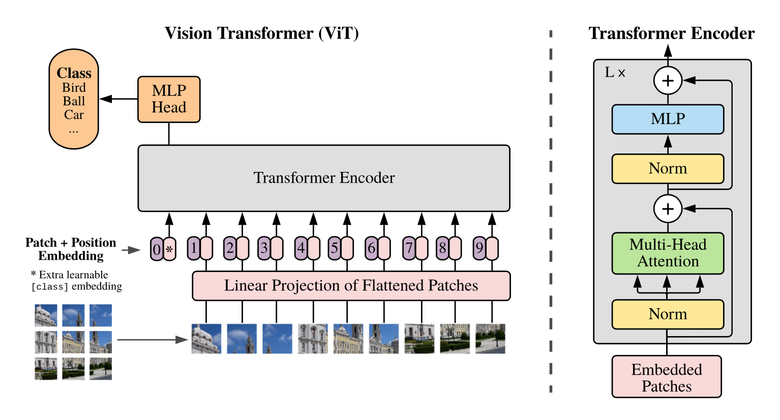
ViT（vision transformer）是Google在2020年提出的直接将transformer应用在图像分类的模型，后面很多的工作都是基于ViT进行改进的。ViT的思路很简单：直接把图像分成固定大小的patchs，然后通过线性变换得到patch embedding，这就类比NLP的words和word embedding，由于transformer的输入就是a sequence of token embeddings，所以将图像的patch embeddings送入transformer后就能够进行特征提取从而分类了。ViT模型原理如下图所示，其实ViT模型只是用了transformer的Encoder来提取特征（原始的transformer还有decoder部分，用于实现sequence to sequence，比如机器翻译）。下面将分别对各个部分做详细的介绍。

Patch Embedding

对于ViT来说，首先要将原始的2-D图像转换成一系列1-D的patch embeddings，这就好似NLP中的word embedding。输入的2-D图像记为 $x\in \mathbb{R}^{H\times W\times C}$，其中 $H$ 和 $W$ 分别是图像的高和宽，而$C$为通道数对于RGB图像就是3。如果要将图像分成大小为 $P\times P$的patchs，可以通过reshape操作得到a sequence of patchs：$x_p\in\mathbb{R}^{N\times(P^2\cdot C)}$，图像共切分为 $N=HW/P^2$ 个patchs，这也就是sequence的长度了，注意这里直接将patch拉平为1-D，其特征大小为 $P^2\cdot C$。然后通过一个简单的线性变换将patchs映射到 $D$ 大小的维度，这就是patch embeddings：$x_p^{'}\in \mathbb{R}^{N\times D}$，在实现上这等同于对 $x_p$ 进行一个 $P\times P$ 且stride为 $P$ 的卷积操作（虽然等同，但是ViT其实是不包含任何卷积操作的），下面是具体的实现代码：

class PatchEmbed(nn.Module):
    """ Image to Patch Embedding
    """
    def __init__(self, img_size=224, patch_size=16, in_chans=3, embed_dim=768):
        super().__init__()
        img_size = to_2tuple(img_size)
        patch_size = to_2tuple(patch_size)
        num_patches = (img_size[1] // patch_size[1]) * (img_size[0] // patch_size[0])
        self.img_size = img_size
        self.patch_size = patch_size
        self.num_patches = num_patches

        self.proj = nn.Conv2d(in_chans, embed_dim, kernel_size=patch_size, stride=patch_size)

    def forward(self, x):
        B, C, H, W = x.shape
        # FIXME look at relaxing size constraints
        assert H == self.img_size[0] and W == self.img_size[1], \
            f"Input image size ({H}*{W}) doesn't match model ({self.img_size[0]}*{self.img_size[1]})."
        x = self.proj(x).flatten(2).transpose(1, 2)
        return x

Position Embedding

除了patch embeddings，模型还需要另外一个特殊的position embedding。transformer和CNN不同，需要position embedding来编码tokens的位置信息，这主要是因为self-attention是permutation-invariant，即打乱sequence里的tokens的顺序并不会改变结果。如果不给模型提供patch的位置信息，那么模型就需要通过patchs的语义来学习拼图，这就额外增加了学习成本。ViT论文中对比了几种不同的position embedding方案(如下），最后发现如果不提供positional embedding效果会差，但其它各种类型的positional embedding效果都接近，这主要是因为ViT的输入是相对较大的patchs而不是pixels，所以学习位置信息相对容易很多。

无positional embedding
1-D positional embedding：把2-D的patchs看成1-D序列
2-D positional embedding：考虑patchs的2-D位置（x, y）
Relative positional embeddings：patchs的相对位置
transformer原论文中是默认采用固定的positional embedding，但ViT中默认采用学习（训练的）的1-D positional embedding，在输入transformer的encoder之前直接将patch embeddings和positional embedding相加:

# 这里多1是为了后面要说的class token，embed_dim即patch
self.pos_embed= nn.Parameter(torch.zeros(1, num_patches+ 1, embed_dim))

# patch emded + pos_embed
x = x + self.pos_embed

论文中也对学习到的positional embedding进行了可视化，发现相近的patchs的positional embedding比较相似，而且同行或同列的positional embedding也相近：

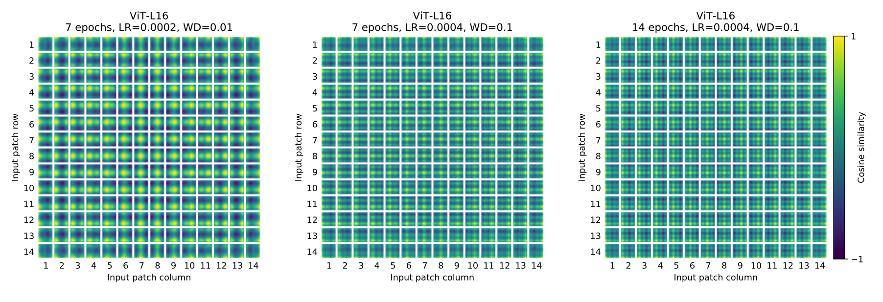
这里额外要注意的一点，如果改变图像的输入大小，ViT不会改变patchs的大小，那么patchs的数量 $N$ 会发生变化，那么之前学习的pos_embed就维度对不上了，ViT采用的方案是通过插值来解决这个问题：

def resize_pos_embed(posemb, posemb_new):
    # Rescale the grid of position embeddings when loading from state_dict. Adapted from
    # https://github.com/google-research/vision_transformer/blob/00883dd691c63a6830751563748663526e811cee/vit_jax/checkpoint.py#L224
    _logger.info('Resized position embedding: %s to %s', posemb.shape, posemb_new.shape)
    ntok_new = posemb_new.shape[1]
    # 除去class token的pos_embed
    posemb_tok, posemb_grid = posemb[:, :1], posemb[0, 1:]
    ntok_new -= 1
    gs_old = int(math.sqrt(len(posemb_grid)))
    gs_new = int(math.sqrt(ntok_new))
    _logger.info('Position embedding grid-size from %s to %s', gs_old, gs_new)
    # 把pos_embed变换到2-D维度再进行插值
    posemb_grid = posemb_grid.reshape(1, gs_old, gs_old, -1).permute(0, 3, 1, 2)
    posemb_grid = F.interpolate(posemb_grid, size=(gs_new, gs_new), mode='bilinear')
    posemb_grid = posemb_grid.permute(0, 2, 3, 1).reshape(1, gs_new * gs_new, -1)
    posemb = torch.cat([posemb_tok, posemb_grid], dim=1)
    return posemb

但是这种情形一般会造成性能少许损失，可以通过finetune模型来解决。另外最新的论文CPVT通过implicit Conditional Position encoding来解决这个问题（插入Conv来隐式编码位置信息，zero padding让Conv学习到绝对位置信息）。

Class Token

除了patch tokens，ViT借鉴BERT还增加了一个特殊的class token。后面会说，transformer的encoder输入是a sequence patch embeddings，输出也是同样长度的a sequence patch features，但图像分类最后需要获取image feature，简单的策略是采用pooling，比如求patch features的平均来获取image feature，但是ViT并没有采用类似的pooling策略，而是直接增加一个特殊的class token，其最后输出的特征加一个linear classifier就可以实现对图像的分类（ViT的pre-training时是接一个MLP head），所以输入ViT的sequence长度是 $N+1$。class token对应的embedding在训练时随机初始化，然后通过训练得到，具体实现如下：

# 随机初始化
self.cls_token = nn.Parameter(torch.zeros(1, 1, embed_dim))

# Classifier head
self.head= nn.Linear(self.num_features, num_classes) if num_classes> 0 else nn.Identity()

# 具体forward过程
B= x.shape[0]
x= self.patch_embed(x)
cls_tokens= self.cls_token.expand(B,-1,-1)# stole cls_tokens impl from Phil Wang, thanksx= torch.cat((cls_tokens, x), dim=1)
x= x+ self.pos_embed

Transformer Encoder

transformer最核心的操作就是self-attention，其实attention机制很早就在NLP和CV领域应用了，比如带有attention机制的seq2seq模型，但是transformer完全摒弃RNN或LSTM结构，直接采用attention机制反而取得了更好的效果：attention is all you need！简单来说，attention就是根据当前查询对输入信息赋予不同的权重来聚合信息，从操作上看就是一种“加权平均”。attention中共有3个概念：query, key和value，其中key和value是成对的，对于一个给定的query向量 $q\in\mathbb{R}^d$，通过内积计算来匹配k个key向量（维度也是$d$，堆积起来即矩阵 $K \in\mathbb{R}^{k\times d}$），得到的内积通过softmax来归一化得到 $k$ 个权重，那么对于query其attention的输出就是k个key向量对应的value向量（即矩阵 $V \in \mathbb{R}^{k\times d}$）的加权平均值。对于一系列的 $N$ 个query（即矩阵 $Q\in\mathbb{R}^{N\times d}$ ），可以通过矩阵计算它们的attention输出：

这里的 $\sqrt{d_k}$ 为缩放因子以避免点积带来的方差影响。上述的Attention机制称为 Scaled dot product attention，其实attention机制的变种有很多，但基本原理是相似的。如果 $Q,K,V$都是从一个包含 $N$ 个向量的sequence（ $X\in \mathbb{R}^{N\times D}$ ）通过线性变换得到：$Q = XW_Q,K=XW_K,V+XW_V$ 那么此时就变成了 self-attention，这个时候就有 $N$ 个（key,value）对，那么$k=N$ 。self-attention是transformer最核心部分，self-attention其实就是输入向量之间进行相互attention来学习到新特征。前面说过我们已经得到图像的patch sequence，那么送入self-attention就能到同样size的sequence输出，只不过特征改变了。

更进一步，transformer采用的是 multi-head self-attention (MSA），所谓的MSA就是采用定义 $h$ 个attention heads，即采用 $h$ 个self-attention应用在输入sequence上，在操作上可以将sequence拆分成$ h$ 个size为 $N\times d$ 的sequences，这里 $D = hd$，$h$ 个不同的heads得到的输出concat在一起然后通过线性变换得到最终的输出，size也是 $N\times D$：

MSA的计算量是和 $N^2$ 成正相关的，所以ViT的输入是patch embeddings，而不是pixel embeddings，这有计算量上的考虑。在实现上，MSA是可以并行计算各个head的，具体代码如下：

**class** **Attention**(nn**.**Module):
    **def** __init__(self, dim, num_heads**=**8, qkv_bias**=**False, qk_scale**=**None, attn_drop**=**0., proj_drop**=**0.):
        super()**.**__init__()
        self**.**num_heads **=** num_heads
        head_dim **=** dim **//** num_heads

        self**.**scale **=** qk_scale **or** head_dim ****** **-**0.5

        self**.**qkv **=** nn**.**Linear(dim, dim ***** 3, bias**=**qkv_bias)
        self**.**attn_drop **=** nn**.**Dropout(attn_drop)
        self**.**proj **=** nn**.**Linear(dim, dim)
        *# 这里包含了dropout
                *self**.**proj_drop **=** nn**.**Dropout(proj_drop)

    **def** **forward**(self, x):
        B, N, C **=** x**.**shape
        qkv **=** self**.**qkv(x)**.**reshape(B, N, 3, self**.**num_heads, C **//** self**.**num_heads)**.**permute(2, 0, 3, 1, 4)
        q, k, v **=** qkv[0], qkv[1], qkv[2]   *# make torchscript happy (cannot use tensor as tuple)

                *attn **=** (q @ k**.**transpose(**-**2, **-**1)) ***** self**.**scale
        attn **=** attn**.**softmax(dim**=-**1)
        attn **=** self**.**attn_drop(attn)

        x **=** (attn @ v)**.**transpose(1, 2)**.**reshape(B, N, C)
        x **=** self**.**proj(x)
        x **=** self**.**proj_drop(x)
        **return** x

在transformer中，MSA后跟一个FFN（Feed-forward network），这个FFN包含两个FC层，第一个FC层将特征从维度$D$ 变换成 $4D$，后一个FC层将特征从维度$4D$ 恢复成 $D$，中间的非线性激活函数采用GeLU，其实这就是一个MLP，具体实现如下：

**class** **Mlp**(nn**.**Module):
    **def** __init__(self, in_features, hidden_features**=**None, out_features**=**None, act_layer**=**nn**.**GELU, drop**=**0.):
        super()**.**__init__()
        out_features **=** out_features **or** in_features
        hidden_features **=** hidden_features **or** in_features
        self**.**fc1 **=** nn**.**Linear(in_features, hidden_features)
        self**.**act **=** act_layer()
        self**.**fc2 **=** nn**.**Linear(hidden_features, out_features)
        self**.**drop **=** nn**.**Dropout(drop)

    **def** **forward**(self, x):
        x **=** self**.**fc1(x)
        x **=** self**.**act(x)
        x **=** self**.**drop(x)
        x **=** self**.**fc2(x)
        x **=** self**.**drop(x)
        **return** x

那么一个完成transformer encoder block就包含一个MSA后面接一个FFN，其实MSA和FFN均包含和ResNet一样的skip connection，另外MSA和FFN后面都包含layer norm层，具体实现如下：

**class** **Block**(nn**.**Module):

    **def** __init__(self, dim, num_heads, mlp_ratio**=**4., qkv_bias**=**False, qk_scale**=**None, drop**=**0., attn_drop**=**0.,
                 drop_path**=**0., act_layer**=**nn**.**GELU, norm_layer**=**nn**.**LayerNorm):
        super()**.**__init__()
        self**.**norm1 **=** norm_layer(dim)
        self**.**attn **=** Attention(
            dim, num_heads**=**num_heads, qkv_bias**=**qkv_bias, qk_scale**=**qk_scale, attn_drop**=**attn_drop, proj_drop**=**drop)
        *# NOTE: drop path for stochastic depth, we shall see if this is better than dropout here
        *self**.**drop_path **=** DropPath(drop_path) **if** drop_path **>** 0. **else** nn**.**Identity()
        self**.**norm2 **=** norm_layer(dim)
        mlp_hidden_dim **=** int(dim ***** mlp_ratio)
        self**.**mlp **=** Mlp(in_features**=**dim, hidden_features**=**mlp_hidden_dim, act_layer**=**act_layer, drop**=**drop)

    **def** **forward**(self, x):
        x **=** x **+** self**.**drop_path(self**.**attn(self**.**norm1(x)))
        x **=** x **+** self**.**drop_path(self**.**mlp(self**.**norm2(x)))
        **return** x

ViT

对于ViT模型来说，就类似CNN那样，不断堆积transformer encoder blocks，最后提取class token对应的特征用于图像分类，论文中也给出了模型的公式表达，其中

（1）就是提取图像的patch embeddings，然后和class token对应的embedding拼接在一起并加上positional embedding；
（2）是MSA，（3）是MLP，（2）和（3）共同组成了一个transformer encoder block，共有$L$层；
（4）是对class token对应的输出做layer norm，然后就可以用来图像分类。

除了完全无卷积的ViT模型外，论文中也给出了Hybrid Architecture，简单来说就是先用CNN对图像提取特征，从CNN提取的特征图中提取patch embeddings，CNN已经将图像降采样了，所以patch size可以为 $1\times 1$。

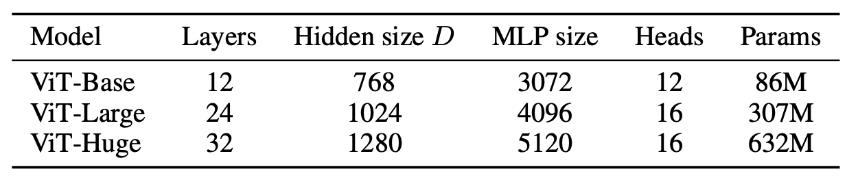
ViT模型的超参数主要包括以下，这些超参数直接影响模型参数以及计算量：

Layers：block的数量；
Hidden size D：隐含层特征，D在各个block是一直不变的；
MLP size：一般设置为4D大小；
Heads：MSA中的heads数量；
Patch size：模型输入的patch size，ViT中共有两个设置：14x14和16x16，这个只影响计算量；
类似BERT，ViT共定义了3中不同大小的模型：Base，Large和Huge，其对应的模型参数不同，如下所示。如ViT-L/16指的是采用Large结构，输入的patch size为16x16。

VIT优势

那么，ViT 模型与 CNN 相比，到底好在什么地方呢？具体来说，有以下六个方面的不同：

（1）从浅层和深层中获得的特征之间，ViT 有更多的相似性；

（2）ViT 表示从浅层获得全局特征；

（3）ViT 中的跳跃连接影响比 CNNs（ResNet）大，且大大地影响特征的表现和相似性；

（4）ViT 保留了比 ResNet 更多的空间信息；

（5）通过大量的数据，ViT 能学到高质量的中间特征；

（6）与 ResNet 相比，ViT 的表示是更接近于 MLP-Mixer。

Reference

"未来"的经典之作ViT：transformer is all you need!